Usage

The Kaipy package comes with a variety of tools to help you load and analyze data from the MAGE model. This page will walk you through the basic usage of the package. This includes using the API to load datasets and create plots as well as using the command line interface to run scripts.

Kaipy API Package

We will go over the basics of loading datasets and creating plots using the Kaipy API package. You can try this out for yourself using our Google Colab notebook.

Loading datasets

In order to load data for the GAMERA and MIX components of the MAGE model you will need to import the following modules:

import kaipy.gamera.magsphere as msph
import kaipy.remix.remix as remix
import os

Start by importing the magnetosphere data. You will need to set the fdir variable to the directory containing the output from a MAGE magnetosphere run. The ftag variable will need to be set to the name that identifies the MAGE ouput. For example

basedir = '/content/gdrive/MyDrive/MAGEColab'
fdir = os.path.join(basedir,'GrossREU')
ftag = 'GrossREUSlim'

Now we use the msph portion of the kaipy package to setup a pipeline to the magnetosphere data. For this example we will set the step we want to display to the final step of the run.

gsph = msph.GamsphPipe(fdir,ftag,doFast=False)
nstep = gsph.sFin

Importing the ionospheric data from REMIX follow the same format as the import of the magnetospheric data with the added requirement of specifying which hemisphere, e.g. NORTH or SOUTH, that you want to plot.

mixFiles = os.path.join(fdir,"%s.mix.h5"%(ftag))
ion = remix.remix(mixFiles,nstep)
ion.init_vars('NORTH')

Plots

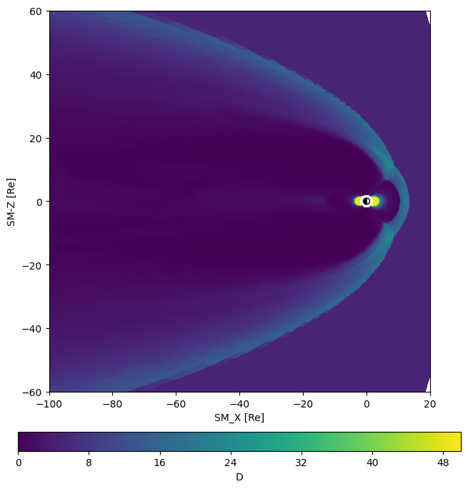
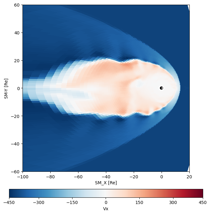
The msphViz portion of the kaipy library has numerous routines for visualizing the magnetosphere. Here will demostrate usage of plotXY and plotXZ which make plots of the equatorial and meridional cuts of the magnetosphere. For both of these routines and others in system you need to provide the instance of the magnetosphere object, the step number you want to display, the extent of the domain, and two sets of axes. The first axes object is for the plot and the second is for the colorbar. For plotXZ we will use the minimal set arguments which results in a plot density. For the plotXY example we will specify options so that we end up with Vx on Red/Blue color palette with a mid point normalization.

First the plotXZ example

xyBds = [-100,20,-60,60]
figSz = (8,8)
fig = plt.figure(figsize=figSz)
gs = fig.add_gridspec(2,1,height_ratios=[20,1],hspace=0.2)
Ax1 = fig.add_subplot(gs[0,0])
AxC1 = fig.add_subplot(gs[1,0])
data = mviz.plotXZ(gsph,nstep,xyBds,Ax1,AxC1,vMin=0,vMax=50)

And for the plotXY example

figSz = (8,8)
fig = plt.figure(figsize=figSz)
gs = fig.add_gridspec(2,1,height_ratios=[20,1],hspace=0.2)
Ax1 = fig.add_subplot(gs[0,0])
AxC1 = fig.add_subplot(gs[1,0])
data = mviz.plotXY(gsph,nstep,xyBds,Ax1,AxC1,var='Vx',midp=True,cmap='RdBu_r')

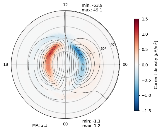
The mix object includes an extensive plotting routine that has the capability for numerous variables with excellent choices for the color tables. It also takes advantage of the mix object’s ability to calculate derived quanties, such as magnetic perturbations and electric fields. Unlike the magnetosphere plotting routines it has the option to take a gridspec object instead of an axes object. It also has the option be made an inset plot so that it can be easily combined with a magnetosphere plot.

ion.plot('current')

Kaipy Command Line Interface

The Kaipy package also comes with a command line interface that allows you to run scripts to analyze MAGE model data. The CLI is a great way to automate the analysis of large datasets. The CLI is run from the terminal and has a variety of options to customize the analysis.

A complete list of the available scripts can be found at the Scripts documentation.

The quicklook directory has numerous scripts that can be used to generate plots and movies of the MAGE model output. For example the msphpic.py command makes a summary movie of the magnetosphere while the mixpic.py command makes a summary movie of the ionosphere.

msphpic.py

Creates simple multi-panel figure for Gamera magnetosphere run Top Panel - Residual vertical magnetic field Bottom Panel - Pressure (or density) and hemispherical insets NOTE: There is an optional -size argument for domain bounds options (default: std), which is passed to kaiViz functions.

usage: msphpic.py [-h] [--debug] [-d directory] [-id runid] [-n step] [-bz]
                  [-den] [-jy] [-ephi] [-noion] [-nompi] [-noIM] [-bigIM]
                  [-src] [-v] [--spacecraft spacecraft] [-vid] [-overwrite]
                  [--ncpus ncpus] [-nohash]
                  [-size {small,std,big,bigger,fullD,dm}]

-h, --help

show this help message and exit

--debug

Print debugging output (default: False).

-d <directory>

Directory containing data to read (default: /home/docs/checkouts/readthedocs.org/user_builds/kaipy-docs/checkouts/latest/docs/source)

-id <runid>

Run ID of data (default: msphere)

-n <step>

Time slice to plot (default: -1)

-bz

Show Bz instead of dBz (default: False).

-den

Show density instead of pressure (default: False).

-jy

Show Jy instead of pressure (default: False).

-ephi

Show Ephi instead of pressure (default: False).

-noion

Don’t show ReMIX data (default: False).

-nompi

Don’t show MPI boundaries (default: False).

-noIM

Don’t show Inner Mag data (default: False).

-bigIM

Show entire Inner Mag domain (default: False).

-src

Show source term (default: False).

-v, --verbose

Print verbose output (default: False).

--spacecraft <spacecraft>

Names of spacecraft to plot positions, separated by commas (default: None)

-vid

Make a video and store in mixVid directory (default: False)

-overwrite

Overwrite existing vid files (default: False)

--ncpus <ncpus>

Number of threads to use with –vid (default: 1)

-nohash

Don’t display branch/hash info (default: False)

-size {small,std,big,bigger,fullD,dm}

Domain bounds options (default: std)

mixpic.py

Creates simple multi-panel REMIX figure for a GAMERA magnetosphere run. Top Row - FAC (with potential contours overplotted), Pedersen and Hall Conductances Bottom Row - Joule heating rate, particle energy and energy flux

usage: mixpic.py [-h] [--debug] [-id runid] [-n step] [-nflux] [-print]
                 [--spacecraft spacecraft] [-v] [-GTYPE] [-PP] [-vid]
                 [-overwrite] [--ncpus ncpus] [-nohash] [--coord coord]

-h, --help

show this help message and exit

--debug

Print debugging output (default: False).

-id <runid>

Run ID of data (default: msphere)

-n <step>

Time slice to plot (default: -1)

-nflux

Show number flux instead of energy flux (default: False)

-print

Print list of all steps and time labels, then exit (default: False)

--spacecraft <spacecraft>

Names of spacecraft to plot magnetic footprints, separated by commas (default: None)

-v, --verbose

Print verbose output (default: False).

-GTYPE

Show RCM grid type in the eflx plot (default: False)

-PP

Show plasmapause (10/cc) in the eflx/nflx plot (default: False)

-vid

Make a video and store in mixVid directory (default: False)

-overwrite

Overwrite existing vid files (default: False)

--ncpus <ncpus>

Number of threads to use with –vid (default: 1)

-nohash

Don’t display branch/hash info (default: False)

--coord <coord>

Coordinate system to use (default: SM)